Can We Improve a Trading Bot Using Machine Learning?

Trading Bots, you might have heard this term at least once.
I’ve recently started my path in becoming a data scientist and of course machine learning and AI are a crucial part of this, Trading has been somewhat of a hobby for me, i have never made this into a career(and i don’t intend to, for the time being) but everyone that has come across this topic has heard about trading bots, an automated way of trading the market, these bots always have a fee for license or monthly subscription service.
Trading bots are not so reliable(or at least, that is the most popular opinion), so now that i have some knowledge on ML, i asked myself:
Is it possible to use ML to predict if this Trading Bot makes the right trade?
and that’s when i got to work!, basically market can only go 2 ways: up or down and traders in different markets can make money both ways(by going long or short, in trading lingo) But, how often do you actually make the right choice is what sets you apart from the bunch!, of course i am not saying that you have to be right 100% of the time (which is impossible statitically)
“In trading, you win by not losing!”
pretty straightforward approach! as said by VP From the No Nonsense forex Youtube Channel so this is going to be our main goal: reducing losses!.
first i needed to find my data! which i sourced from myfxbook.com from there i started to look through and found a good candidate: the Daxbot GBPUSD, for my luck This website kept track of all the trades taken by this bot since 2015 and still is recording all trades taken up until this day! claiming a 70% win rate which is not bad at all! but the question is, can we improve this? challenge accepted
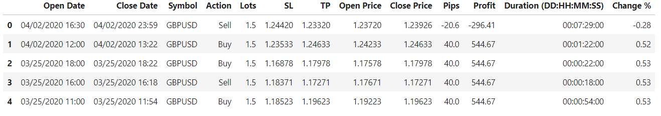
the initial data i gathered was not much to work with most of the features here where unusable to a model…
But did I give up? CLARO QUE NO!.
first i had to make this a classification problem, so made a new feature that would tell me whether a trade was lost or won, i’ve enclosed my data cleaning process on this function below:
def wrangle(x):
    x = x.copy()
    #removing spaces and upper cases
    x.columns = x.columns.str.lower()
    x.columns = x.columns.str.replace(' ','_')

    #engeneering a few features
    x['win/loss'] = x['profit'] > 0 #this feature will determine if there is a winning or losing trade
    features_ = x.loc[:,'sl':'open_price'] #this variable subsets my main columns openprice, stoploss and take profit
    x['mean'] = features_.mean(axis=1)
    x['med'] = features_.median(axis=1)
    x['std'] = features_.std(axis=1)
    multiplier = 0.0001

    x['risk_reward'] = round((x['sl']-x['tp'])/multiplier)

    #dropping some of the features that cause leakage
    x = x.drop(labels=['profit','pips','change_%',"duration_(dd:hh:mm:ss)"],axis=1)

    #setting columns as datetime
    x['open_date'] = pd.to_datetime(x['open_date'])
    x['close_date'] = pd.to_datetime(x['close_date'])
    return x
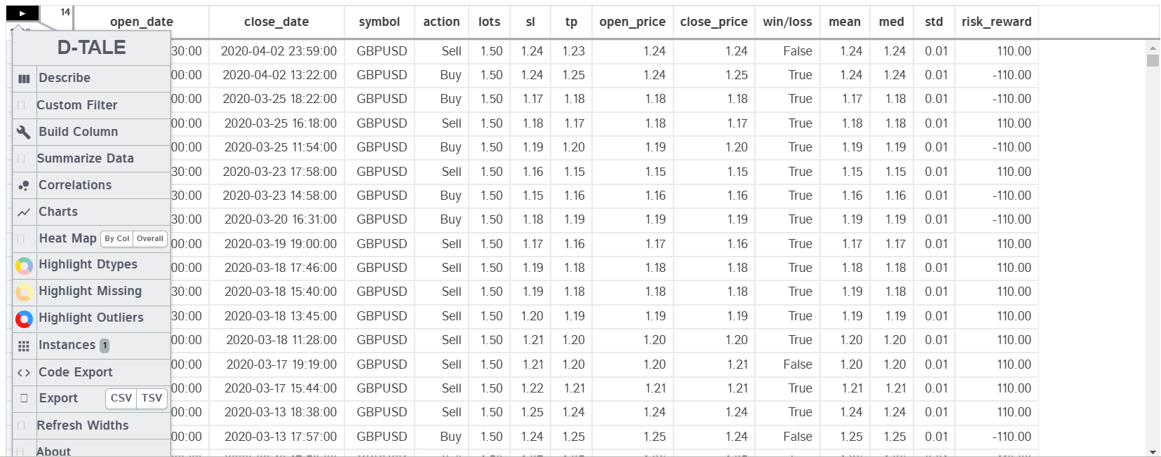
for my data exploration, i used an automated tool called Dtale, recommended to me by one of my classmates you can check it out here!.
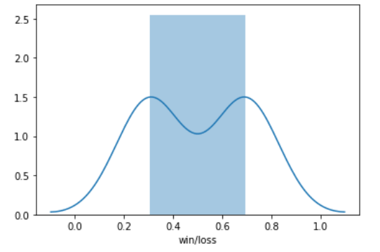
The Classes of the Win loss column(which is our target), its a Boolean data type, if True it means that the trade made profit, otherwise is marked as False. lets check its distribution in numbers:
True     0.695988
False    0.304012
Name: win/loss, dtype: float64
now let’s vizualize it:
i have decided to do a time based split in this problem, since we want to basically predict future actions on the strategy, we can’t let our model see the future(data leakage).
#now lets subset our data into a time based split
#the train set will be data before our cutoff, the test data will be
#data after our cutoff date
cutoff = pd.to_datetime('2018/11/1')#<---cutoff date
train = df[df['open_date']<=cutoff]
test = df[df['open_date']>cutoff]
Here we will start to make a baseline model to try to beat it with a better model. the error metric i chose for this problem is ROC AUC(Reciever Operating Characteristic Area Under the Curve), since this metric actually aims to reduce false positive rates and increase true positives, in trading you definetly want to make the Right decision most of the time.
# now lets subset our data into x and y
# here is our target and features for our classification problem
target = 'win/loss'
features = ['action','sl','tp','open_price','mean','close_price','risk_reward']
X_train = train[features]
y_train = train[target]
X_test = test[features]
y_test = test[target]
some of the libraries:
#lets fit a regular linear regression and use that as our baseline model, then we will try to
#improve it if possible
from sklearn.ensemble import RandomForestClassifier
import category_encoders as ce
from sklearn.pipeline import make_pipeline
from sklearn.linear_model import LogisticRegressionCV, LogisticRegression
So, after fitting the model to a logistic regression(which will be our baseline), i decided to make a cross validation to see the results.
from sklearn.metrics import roc_auc_score
lg_cvscore = cross_val_score(pipeline,X_train,y_train,scoring='roc_auc')
np.mean(lg_cvscore)
>>>0.47302722610756537
About 47% ROCAUC score… we can do better than that, so i decided to fit a Random Forest Classifier to try and get better results.
#Now lets try one of my favorite models: Randomforestclassifier
pipeline_rf = make_pipeline(
    ce.BinaryEncoder(),
    RandomForestClassifier()
)
After Fitting our Train data to the new model we ran another cross validation score:
# now lets see the validation accuracy to see if it improves
rf_cvscore = cross_val_score(pipeline_rf,X_train,y_train,scoring='roc_auc',cv=21)
np.mean(rf_cvscore)
0.8058061482168626
plot of the ROC/AUC line:
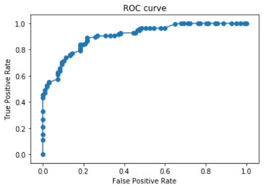
The average ROC score of the Random forest model is 80%! That’s awesome, but we should’nt be celebrating just yet, we have to know why this model is so much better than our baseline model…
Here are the Permutation Importances of the model:
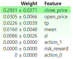
We can notice in the permutation importances that close_price is the most important feature, i also did a Partial Dependence plot just to vizualize the correlation with our target variable:
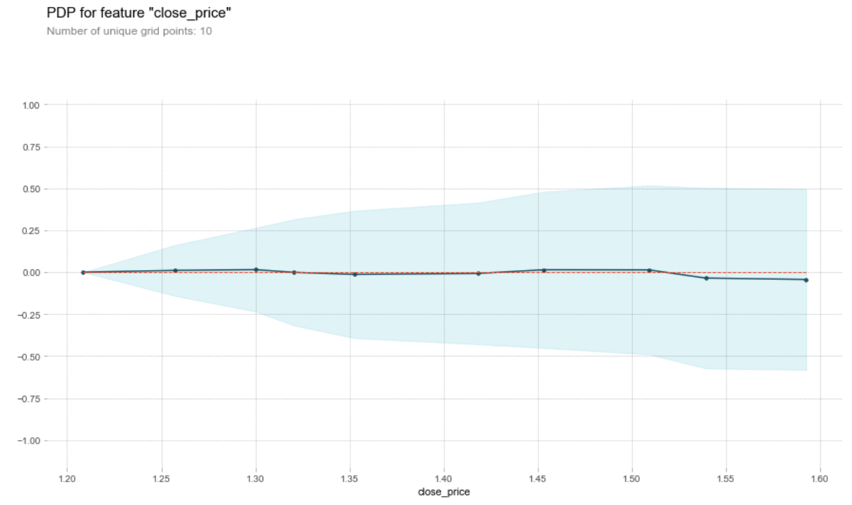
Upon further investigating why this feature was so important i realized that this feature should not be here, when a trader opens a position, whether is buying or selling, we would not know with certainty what the close price is going to be. of course you can provide the desired close price and get a prediction on how likely it would be that your trade is profitable if it closes at that desired price, but anyways i think i can do better!
Now, that did not end my investigation there, i already invested so much time into it, so decided to go an extra mile: creating another model that can predict an aproximate close price for any open trade, and use that into our first model.
# first lets redefine our targets and features
# in this clase Close_price will be our target.
target = 'close_price'
features = ['action','sl','tp','open_price','risk_reward','mean']

X_train = train[features]
y_train = train[target]
X_test = test[features]
y_test = test[target]
Here i decided to make a Ridge Regression model to try and predict our approximate closing price, i tested a couple of models and actually this was the one that had the best results, for this one problem i used Mean Absolute Error as the evaluation metric since it’s a metric that can predict the most minimal change in price, in the case of currency trading, Pips(Percentage in points), is the main metric you go for when measuring your profits or losses. More information on pips here
#this is the pipeline we are going to use
pipeline = make_pipeline(
    ce.BinaryEncoder(),
    Ridge()
)
# then let's fit our model
pipeline.fit(X_train,y_train)

#and the Mean absolute error is...
from sklearn.metrics import mean_absolute_error
mean_absolute_error(y_pred,y_test)
>>>0.004875578794760977
So the Mean absolute error would be around 48 pips, i would like something a little bit more accurate but i will need a more sensitive model to try and get most of the minimal variance in price.
Conclusion
This proyect has really made me feel proud because this problem that i came accross is not the typical problem you see in class since you have to have a general understanding of trading and maybe some of the general rules in Data Science might not apply in this problem to achieve the result i want to get, but anyways, when i think about it, being able to do this much with this little amount of data it’s definetly an acomplishment for me.
i have not given up on this and i will update this post with more information in the future, i will upload my notebook to github so you can check it out too.
Thank you for making it this far!