Naive Bayes Classifier, Simply explained!
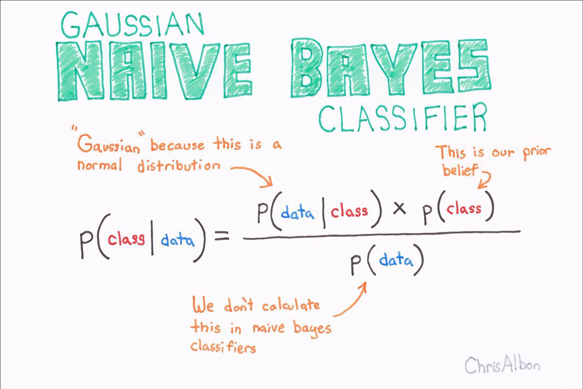
Bayes Theorem and Bayesian statistics is one of the things that i became the most interested in when i first embarked in my Data Science journey early this year, the basics of the Bayes statistics in a nutshell is the fact that everything is the way it is for a reason, and not just because the mean of x is 158. Let’s take a look at what Bayes Theorem actually is about:
| **P(A | B) = P(B | A) * P(A) / P(B)** |
To break it down, the probability of A (a being the Event in question) given B (the evidence of the event) is Equal to the Probability of B given A times the Prior Probability of A divided by the Prior Probability of B.
The way i like to understand stuff is by putting it in terms that i am familiar with, I’ll give you an example and then you can make it your own… i hope.
Let’s say that you are in a very concurred street, and the city that you are in is not very safe, in my case where i am from, I’ve seen a lot of robberies happen from people who are in a motorcycle, and almost every time i see someone in a motorcycle i tend to stay alert (Dominicans know what i am talking about), but, what is the actual probability that someone is a thief given that he is in a motorcycle in this street? First we have to consider how many people are in this street and how many of them are riding a motorcycle, and what is the chance of a person being a thief in the first place?
| **P(Thief | riding a motorcycle)** |
Let’s say there are 50 people in this street altogether, 20 are riding a motorcycle, 30 are not, like i said before, when someone is in a motorcycle people tend to get scared, so let’s say that 3 people out of the ones who are riding a bike are actually thieves, vs maybe 1 out of the people who are not riding a bike are actual thieves…
let’s get the probability of a Thief being in a motorcycle:
| **P(Thief | riding a motorcycle) = 3 / 20** |
| **P(Thief | riding a motorcycle) = 0.15** |
The 0.15 value that we got is what is called a Probability, this is a guess that we made based on the estimations of the amount of potential thieves given that they are riding a motorcycle.
Now let’s do the same for people who are not in a motorcycle:
| **P(Thief | Not in a Motorcycle) = 1 / 30** |
| **P(Thief | Not in a Motorcycle) = 0.03** |
So in this case the Probability for a person to be a thief is 0.03 if they are not in a motorcycle.
now let’s calculate what is called the Prior Probability, this is a value of a person being a thief in a motorcycle or not taking in consideration the total amount of possible thieves in the sample size.
P(In a Motorcycle) = 3 / 3 + 1
P(In a Motorcycle) = 3 / 4
P(In a Motorcycle) = 0.75
Prior Probability of a thief on a motorcycle is 0.75, we get this number by dividing the number of thieves in a motorcycle by the sum of the number of thieves in a motorcycle and the ones that were not in one. We do the same for the opposite case.
P(Not in a Motorcycle) = 1 / 1 + 3
P(Not in a Motorcycle) = 1 / 4
P(Not in a Motorcycle) = 0.25
So now we need to get the initial probabilities and the Prior probabilities and multiply everything and see what we get…
-probability of a thief being in a motorcycle multiplied by the Prior Probability
| **P(Thief | In a Motorcycle) =0.15** |
P(In a Motorcycle) = 0.75
0.15 X 0.75 =0.11
-probability of a thief NOT being in a motorcycle multiplied by the Prior Probability.
| **P(Thief | Not in a Motorcycle) = 0.03** |
P(Not in a Motorcycle) = 0.25
0.03 X 0.25 = 0.0075
Now since 0.11 is greater than 0.0075 we can assume that is more likely that a thief is going to be in a motorcycle!
Of course this is a very simple example to understand the intuition behind the theorem, but another question some people may ask is, Why is it called “Naive” Bayes Classifier?!, seems to be a pretty good theorem! , actually this method of classification has high Bias, because when additional information is given to the theorem(Features in Machine Learning lingo) the order of the information given does not matter, since it only computes the probabilities and Prior probabilities to make its predictions, but in application the theorem gives good results overall so it has low Variance.
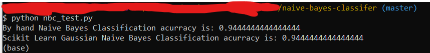
So i implemented some python code based on this theorem from scratch, of course you can always use the Sci kit Learn library to use this and any other model that you like, however doing this by hand really gives you a deeper understanding of how the computer works with this Bayesian method you can find the code here.
i used the built in wine data set to see if i had coded everything correctly and it worked! The accuracy of the handwritten model is the same as the one provided in sci kit learn.
Conclusion
It was a great learning experience doing all the research by hand to have a better grasp of what is going on under the hood of a certain model and being able to speak about it more confidently, i am planning to do another model by hand so stay tuned! I’m open to any suggestions you can get in touch with me via LinkedIn.